Usage
Organizing the data
To use Svetlana, your image(s) first need to be segmented using an external tool such as CellPose, Stardist,… Each Region Of Interest ROI) of the segmentation mask must be given a unique integer value (label), so as to making it possible to identify them.
Once you segmented your data, it must be organized in a specific way:
Parent Folder
├── Images
│   ├── image1
│   ...
│   └── imageN
├── Masks
│  ├── mask1
│   ...
│  └── maskN
The Parent Folder name does not matter, but the subfolder Images and Masks must absolutely be called this way. The prefix ‘image’ and ‘mask’ can also be changed.
The Annotation module
The labeling
Once the dataset is well organized, we can start labeling.
First, the data must be loaded, loading the parent folder. Be careful, it is not possible to drag and drop the folder into Napari to load the data. Then, a patch size around the ROI must be chosen (the bigger the more contextual information). This patch size can be either automatically estimated, based on the biggest ROI in the mask, or set by the user. Be careful with this feature, as if you have a huge outlier in your segmentation mask, this optimal patch size is obviously going to be too large.
Finally, there are two ways to label, whatever the type of image (2D, 3D etc).
Letting Svetlana propose patches one after another in a random order (default way).
Clicking on the objects. For that, activate the option ticking the corresponding case.
In all cases, the labels must be typed on the keyboard. There can be up to 9 classes. The user can set number of classes he wants to deactivate all the other buttons. .. For example, if you work on a 2-class problem, then set the class number to 2, and all the other numbers from 3 to 9 won’t work. This maximum number can be changed at any time during labeling.
If you make a mistake, you can cancel and go back to the previous ROI by clicking “R” on the keyboard.
Saving the result
Once you want to stop labeling you can click on the save the result button to create a binary file called labels. It will be stored in the folder Parent Folder -> Svetlana.
Resuming labeling
You may want to improve your classifier by adding more annotations to your dataset. In that case, you can resume labeling through the dedicated button. You will need to select the Parent Folder again that should contain the folder Svetlana.
If a training and a prediction have already been performed, it will also load a mask of predictions. This allows the user to specifically annotate the wrong predictions. Moreover, a “confidence” mask containing the prediction probability for each ROI can be generated by the user at prediction time. This allows to add a coloured overlay varying from blue (low confidence) to red (high confidence). The blue ROI can be annotated with higher priority to help the neural network better characterizing the objects.
Training
Data loading
By default, the annotations that have just been saved will be opened in this module. It is also possible to use the load data button to load a specific folder with a binary file containing the labels.
Choosing the NN
First choose 2D or 3D to get the appropriate list of neural network architectures. Then pick the architecture you like the best. For most tasks, we advise the use of a simple network such as ‘light_NN_3_5’ or ‘light_NN_3_4’
Classes unbalance
In certain circumstances, it can be impossible to get a balanced dataset, which means approximately the same number of labels for each class. A tick case makes it possible to weight the loss to compensate this phenomenon.
The optimization parameters
The main parameters (number of epochs, learning rate, batch size) are available in the GUI. If you want to use additional features, a JSON configuration file is present in the folder called Svetlana (created in the parent folder). You can change the decay parameters of the learning rate as well as the weights decay of ADAM optimizer.
The data augmentation (optional)
A simple data augmentation based on rotations is available. It is possible to use a much wider panel of transformations using the configuration file. The available features are the ones from the Albumentations library. Please refer to the documentation, for more details. You just need to add the parameters you want to the JSON configuration file.
Example:
Gaussian blurring in documentation :
GaussianBlur(blur_limit=(3, 7), sigma_limit=0, always_apply=False, p=0.5)
Equivalent in JSON configuration file:
"GaussianBlur": {
      "apply": "True",
      "blur_limit": "(3, 7)",
      "sigma_limit": "0",
      "p": "0.5"
  }
where _apply_ indicates whether you want this data augmentation to be applied or not.
Adjusting the contextual information (optional, but crucial)
As illustrated in the companion paper, it is possible to reduce the contextual information around the object in the patch. To do so, we dilate the segmentation mask and multiply the result with the patch (see the paper for more details). This can be set in the configuration file setting the “dilate_mask” option to True. Moreover, the user can choose the size of the structural element for the dilation in pixels/voxels. Obviously, the larger it is, the more contextual information is allowed.
Although optional, this functionality is extremely important, as depending on your application it can be crucial to achieving good results. For instance, in case you want to discriminate between objects that are very close to each other, we strongly recommend the use of this feature.
"dilation": {
            "dilate_mask": "False",
            "str_element_size": "10"
        }

Without multiplying by dilated mask

Multiplying by dilated mask
Transfer learning
If you don’t want to train a neural network from scratch, but rather improve an existing model you can use the ‘load custom model’ button. Note that only PyTorch models can be loaded. Sorry for the TensorFlow fans.
Prediction
Neural network loading
The ‘Load network button’ asks the user to choose the weights file of the training the user wants to use. By default, the weights and network saved in the previous training will be used.
Data loading
Choose the parent folder containing the images to process. By default, the folder which has just been chosen for the labelling and the training will be used.
Note that drag and drop option does not exist for either data or network. Thus, we recommend that you either put the images to be processed with the training images, or create a folder on the same model as the training folder (Images, Masks), containing the images to be processed. In the second case, this folder must be loaded manually using the button provided for this purpose (load data).
Choice of the batch size
This variable defines how many patches are going to be processed at the same time (parallelization), in order to reduce the computing times. Obviously, the more memory your GPU has, the larger this parameter can be chosen.
Prediction of an image
You can choose to predict only the image you are visualizing. Therefore, the prediction mask is going to be displayed. You can tick a case to also provide confidence masks explained above. Once the classification has been processed, you can click on save objects statistics to generate a xlsx file containing morphological features of the classified objects in this image.
Prediction of a batch of images
You can choose to predict the whole folder. Therefore, no result is going to be displayed, but all the results will be stored in a folder called Predictions. You can also tick a case to predict the confidence masks for the whole folder.
Once the entire folder has been processed, a xlsx file containing morphological features of each classified object is generated in the folder called Svetlana.
Saving a mask for each label
A dedicated button computes a mask for each label, i.e. for a 2-class problem, it will generate a mask of objects labeled 1 and another one for objects labeled 2.
Interpretation module of the result
Thanks to the Grad-CAM method, if the corresponding case is checked, it is possible to obtain an interpretation of the way the network makes its decision, by displaying the pixels as a heat map. Indeed, the locations of the pixels that were the most decisive are highlighted (warm colors). Also, for 2D images only, a Grad-CAM variant called guided Grad-CAM is available. It is a combination of edges and grad-CAM (see paper for more details). Both methods are computed at the same times and shown in two different overlays.
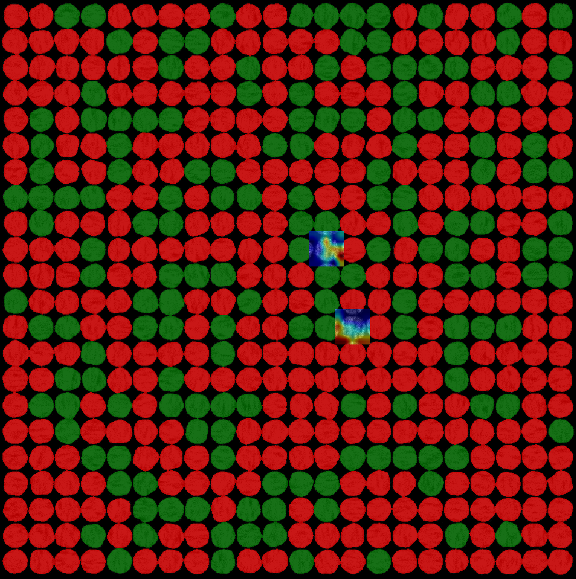
Grad-CAM example
While the case is checked, the user can click on as many cells as he/she wants.